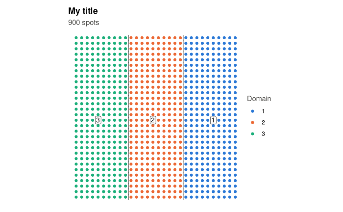
plot(fit, type = ...) draws one of four plots of a sigdots() result: a map of the
domains, a map of the candidate domains, the split tree, or the spatial correlation
estimated at a test. Each plot is a ggplot2 object, so titles, colours and themes can be
changed by adding to it as usual, and it can be saved with ggplot2::ggsave().
Arguments
- x
A result of
sigdots().- type
Which plot to draw, one of:
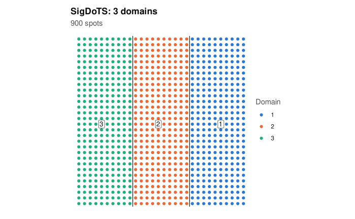
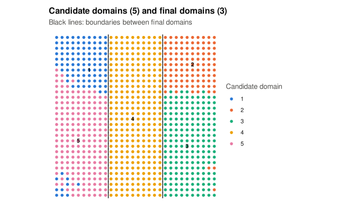
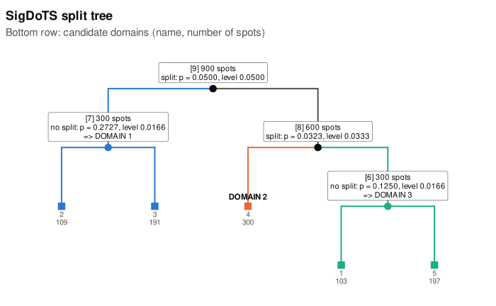
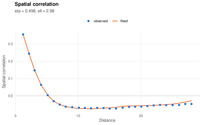
"domains"(the default): a map of the spots at their coordinates, each coloured by its domain, with the domain numbers and the boundaries between domains drawn in. Spots in a part of the tree that could not be tested are grey."candidates": the same map coloured by candidate domain, with the boundaries of the final domains drawn in, so that you can see which candidate domains were merged."tree": the split tree, asprint(x)shows it, as a diagram: every tested part with its decision, p-value and level; the parts that became domains in the colours of"domains"; the candidate domains along the bottom."correlogram": for one test (test), the spatial correlation of the noise, as SigDoTS estimated it for the single-domain model of that test. The points are the correlation between pairs of spots at each distance, after removing each candidate domain's mean and averaged over genes; the line is the correlation the fitted model gives (etais the share of the noise variance that is spatially correlated,ellhow far the correlation reaches). Distances are in units of the typical distance between neighbouring spots. The line following the points means the model describes the spatial correlation of the data.
- test
For
"correlogram": the node number of a tested part, as shown in brackets byprint(x)and in thenodecolumn ofsummary(x)$tests.NULL(the default) means the first test, at the top of the tree. A part that was not tested has no correlogram and gives an error that lists the tested nodes.- point_size
For the two maps: the size of the points, a positive number.
NULL(the default) means45 / sqrt(number of spots), kept between 0.2 and 3.- ...
Not used.
Details
The maps draw each spot at its coordinates with equal scales on the two axes, and the y axis
pointing upwards. Image coordinates (such as the pixel rows of a Visium image) count
downwards, so a map may appear upside down compared with the tissue image; add
ggplot2::scale_y_reverse() to turn it. Domains are coloured in the order of their numbers
with a fixed palette of eight colours (more domains use grDevices::hcl.colors()); the
boundaries are drawn between neighbouring spots of different domains. Each domain's number
is written inside the domain, not on a boundary: for every spot of the domain, the distance
to the nearest spot of another domain (or untested spot) or to the edge of the tissue is
measured, and among the spots where it is at least three quarters of its largest value, the
number goes to the one nearest the domain's mean position. A domain in several separate
pieces is numbered once. The candidate map numbers its candidate domains in the same way.
In the correlogram, points close to the line mean that the single-domain model describes the spatial correlation of the data at that test; points well above the line at short distances mean the model has less spatial correlation than the data, which can make splits easier to keep.
See also
summary.sigdots() for the tests as a table, domains() for the domain of every
spot.